Spectral Library Optimization
The Spectral Library Tool includes three basic library pruning techniques: EMC, IES and CRES. EMC and IES rely on a square array. This is implemented in the background, however the option is left to the user to explore this square array, in order to get a better understanding of the inner workings of IES and EMC.
Square Array
A square array is a way of storing how a specific endmember performs when used to unmix all other spectra in the same library.
A square array is an image of n by n pixels, with n being the number of spectra in the Spectral Library. In this square array, a row corresponds to a spectrum (row = model) used to unmix all other spectra in the library (columns).
The square array is used to store metrics needed for EAR, MASA, CoB and IES. The original format of the square array was proposed by Roberts et al. [Roberts1997] and included in several theses published at UCSB ([Gardner1997], [Halligan2002]).
Square arrays are stored as an ENVI image, with the following possible bands: RMSE, Spectral Angle, Endmember Fraction, Shade Fraction and a ‘Constrained’ band which indicates if the model met the constraints used.
The diagonal represents each spectrum modelling itself and is meaningless so it has been zeroed out for all output bands.
A detailed description of the Square Array Output Bands
RMSE
The RMSE at row A and column B is the root mean square error of spectrum A modelling spectrum B. RMSE is calculated using the following equation:
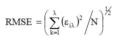
RMSE images are not symmetrical about the diagonal (see endmember fraction description below).
Note
The % RMSE is independent of the reflectance scale factor (1, 1000 or 10000), because all data is converted to values between 0 and 1 before Square Array calculations.
Spectral Angle
Spectral Angle at row A and column B is the angular distance, in radians, between spectrum A and spectrum B. This is the same metric used by ENVI’s Spectral Angle Mapper (SAM) and is calculated as:
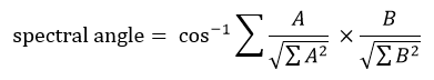
Where A and B are vectors containing the spectral data for spectrum A and B
For spectral angle, the square array will be symmetrical about the diagonal.
Endmember Fraction
The endmember fraction band at row A and column B is the SMA fraction for endmember A when used to model spectrum B.
These images are not symmetrical about the diagonal, because brightness differences contribute to differences in SMA fractions and model RMSE. When bright spectrum A models dark spectrum B the SMA fraction will be between 0 and 100%, and the RMSE will be calculated as the difference between the spectra at the brightness of the darker spectrum B. When dark spectrum B models bright spectrum A the SMA fraction will be greater than 100% and the RMSE will be calculated from the difference between the spectra at the brightness of the brighter spectrum A, and thus will be a larger RMSE than the previous case.
Shade Fraction
The shade fraction at row A and column B is the SMA shade fraction for endmember A when used to model spectrum B. It is calculated as 1 minus the endmember fraction, and is included to allow for shade thresholding in the EMC calculations.
Constraint Code
When calculating the fractions and RMSE, constraints can be used.
Unconstrained: It is allowed to have super positive (>100%) or negative (<0%) fractions or high RMSE values. There will be no ‘constraints’ band in the output.
Constrained, non-reset: Thresholds can be set for minimum and maximum fractions and for RMSE. When either the fractions or the RMSE are exceeded, a value is stored in the ‘constraints’ band (see below). The fractions and RMSE themselves stay unchanged.
Default values of -0.05, 1.05 and 0.025 for minimum fraction, maximum fraction and RMSE threshold, respectively, represent values used in the literature ([Halligan2002], [Roberts2003]).
The minimum fraction constraint cannot be set below -0.50, the maximum fraction constraint cannot exceed 1.50, and the maximum RMSE constraint cannot exceed 0.10.
Constrained, reset: When fractions exceed the constraint, the fractions in the output are reset to the threshold values. The RMSE is then calculated with these new fraction values instead of the original ones. The ‘constraints’ band now stores different values.
This is useful for allowing models with very good fit to be included despite being slightly too dark. For example, spectrum A might be a well-fit spectrum for modelling spectrum B, but would produce a fraction of 106% (1.06) because it is darker than spectrum B. If running in non-reset mode with the maximum allowable fraction set to 105% (1.05), this model would be excluded completely because it exceeds the threshold. In reset mode this model would be run forcing the bright endmember to have a 105% fraction. The resulting RMSE would be slightly higher (due to a slight underestimate of the bright endmember fraction) but would not be excluded. It may even be possible that spectrum A will produce the lowest EAR value for the library, suggesting it is an optimal endmember despite the fact that it is fairly dark.
An overview of the possible values of the constraints band.
- 0 = no constraint breach
- 1 = fraction constraint breach + fraction reset + no RMSE constraint breach
- 2 = fraction constraint breach + no fraction reset + no RMSE constraint breach
- 3 = no fraction constraint breach + RMSE constraint breach
- 4 = fraction constraint breach + fraction reset + RMSE constraint breach
- 5 = fraction constraint breach + no fraction reset + RMSE constraint breach
EAR, MASA, CoB (EMC)
We use the Square Array to determine which spectra within a group of spectra are most representative of their class while covering the range of variability within the class. There are three approaches to do this:
Count based Endmember selection (CoB) was first proposed by Roberts et al. [Roberts2003]. Optimal endmembers are selected as those members of a library that model the greatest number of spectra within their class. Candidate models are assessed by whether they meet fraction and RMSE constraints when unmixing other spectra in the library (stored in the Square Array constraints band).
- The metric in_CoB stores the total number of spectra modelled within the class.
- The metric out_CoB stores the total number of spectra modelled outside of the class
The optimum model is selected as the one that has the highest in_CoB value. Note that ties are not split in this process, so several spectra can have the same in_CoB value.
To determine additional CoB selections, the Spectral Library Tool implements the approach described by Clark [Clark2005]: once an initial optimal spectrum (or spectra, in the case of ties) is selected, all members of the spectral library that were successfully modelled by this spectrum/spectra are culled from the list of candidate CoB spectra. After culling, a second tier in_CoB is calculated and a second tier, optimal spectrum/spectra is selected. This process continues until all candidate spectra have been eliminated, either by being selected as an optimal spectrum or by being modelled by an optimal spectrum.
Out_CoB provides a measure of confusion between classes, with a high value suggesting significant confusion between classes. Ideally, the perfect spectrum will only model members of its class, and not model members outside of its class. This model would have a high in_CoB, but low out_CoB.
To assess the generality of a spectrum we include a third performance metric, the Count Based Index (CoBI) [Clark2005]. CoBI is the ratio of in_CoB to out_CoB with the denominator multiplied by the number of spectra within a class.
Thus a high CoBI and a high in_CoB represents an excellent choice (A specialist as described by Roberts et al. [Roberts1997]. A high CoBI and moderately low in_CoB may also be a good candidate because it captures a member of a class that is spectrally unique, even if it is not well represented in the library. Low values of CoBI would only be acceptable if they were paired with a high in_CoB (Generalists).
Endmember Average RMSE (EAR) was first proposed by Dennison and Roberts [Dennison2003] as a means of locating spectra within a class that provide the best fit when modelling that class. EAR is the average RMSE produced by a spectrum when it is used to model all other members of the same class. The optimum spectrum would be the one that produces the lowest average RMSE.
Minimum Average Spectral Angle (MASA) [Dennison2004] is similar to EAR in that it is designed to select spectra with the best average fit within a class. It differs from EAR in that the measure of fit used is the spectral angle, not the RMSE.
MASA within a class is calculated as the average spectral angle between a candidate model and all other spectra within the same class. The best MASA candidate produces the lowest average spectral angle.
EAR and MASA are conceptually very similar. However, the optimum endmember selected by each metric will depend on the overall brightness of the library. For example, for dark objects, subtle spectral differences between the reference and non-reference spectra could result in a fairly large spectral angle. At the same time, these subtle spectral differences would result in a small RMSE. The net result is that MASA will be far more sensitive to spectral differences for dark objects. For bright objects, the opposite is true. In this case, even a fairly large spectral feature may produce a small difference in spectral angle, but a large difference in RMSE, and EAR would be more sensitive to spectral differences. For further discussion of the differences between RMSE and spectral angle as metrics of spectral fit see Dennison et al [Dennison2004]. Despite differing sensitivities for darker and brighter endmembers, one endmember will frequently possess both the minimum EAR and MASA values.
Note: The strength of any particular selection technique will vary with the metadata field. For example, whereas EAR or MASA may outperform CoB for homogeneous selection criteria, such as dominant, CoB may outperform these measures for heterogeneous selection criteria, such as impervious/pervious. Calculating the EMC file is also critical when choosing the hierarchical level for your selections. For example, if a user were most interested in separating impervious from pervious surfaces, they might opt to sort on impervious/pervious when creating the EMC file. A different user might be interested in separating urban materials, and thus would sort on the material scale.
Iterative Endmember Selection (IES)
Iterative Endmember Selection (IES) is a semi-automated approach for selecting optimal endmember subsets. IES was originally proposed by Schaaf et al. [Schaaf2011] then updated by Roth et al. [Roth2012]. The basic concept of IES is to identify the subset of spectra within a spectral library that provide the best class separability when MESMA is used as a two-endmember classifier. IES operates by first identifying the spectrum within a library that provides the highest classification accuracy as quantified using the kappa coefficient. This endmember would belong to the most commonly represented class in the library. Next, it identifies the endmember which, in combination with the first choice, generates the highest kappa. In the next iteration, it repeats, adding a third endmember. As it continues to iterate, it also tests all previous endmember selections to determine whether removing an endmember increases kappa. IES continues to iteratively add, and subtract spectra until the kappa coefficient no longer improves.
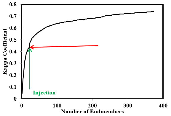
The Spectral Library Tool also includes a modified form of IES, called Forced IES, in which rare endmembers can be identified in a library. Forced IES, which was originally proposed by Roth et al. [Roth2012], is needed when an endmember class is rare, but also important. Because it is rare, IES does not identify an endmember belonging to the class if it results in a decrease in kappa. You can use another endmember selection tool, such as EMC, to identify the best representative spectra from the rare class. One or more of these user-selected endmembers is then injected into the endmember selection process after a set number of iterations, forcing IES to identify an optimal subset that also includes the forced endmembers. As shown below, initially forcing the endmember results in a decrease in Kappa, but IES rapidly identifies models that increase accuracy, iterating until accuracy no longer improves. IES tends to generate much larger spectral libraries than EMC, but also results in higher classification accuracies.
IES was used by Roberts et al. ([Roberts2012]; [Roberts2017]) to discriminate urban surface materials, map plant species and estimate fractional cover in the Santa Barbara area, using MASTER to evaluate the relationship between cover, species and land surface temperature ([Roberts2015]). Other applications of IES included creating multi-temporal libraries for mapping vegetation species ([Dudley2015]) and improved mapping of fire severity ([Fernandez2016]; [Quintano2017]). Roth et al. [Roth2015] evaluated the performance of IES across a diversity of North American ecosystems, finding that Linear Discriminant Analysis (LDA) using Canonical Discriminant Analysis (CDA) was a superior classifier, but MESMA classification results could be improved using dimensionality reduction, such as CDA.
Constrained Reference Endmember Selection (CRES)
The CRES module represents an alternative approach to endmember selection. With CRES a user supplies expert knowledge on the expected SMA fractions at a particular location in order to select the optimal endmembers for that site. This approach was first described by Roberts et al. [Roberts1993] and later discussed in more detail in Roberts et al. [Roberts1998]. It has been used extensively in a number of papers published out of the VIPER group to select optimum endmembers for simple spectral mixture analysis ([Roberts2002], [Roberts2004]). CRES is a tool that aids the user to see which endmembers will produce SMA fractions that produce the closest match to the estimated fractions.
MUSIC
Unlike IES, MUSIC by [Iordache2014] is an image-based library pruning method designed to select, from a large library, a subset of pure spectra that best represents the spectral variability of a given hyperspectral image and that, as a consequence, constitutes the best input for subpixel fractional abundance estimation.
MUSIC essentially comprises two steps. Firstly, the hyperspectral image is represented as a small set of eigenvectors that together define the image subspace, the n-dimensional space in which the data “live”. This step is accomplished using the HySime algorithm ([BioucasDias2008]), which needs no input parameters and estimates the required number of eigenvectors (k) based on the signal- and noise correlation matrices of the original image.
Secondly, the Euclidean distances between each library spectrum and the estimated image subspace are calculated through orthogonal projection. The resulting projection errors, or distances between library members and image, are sorted and the spectra corresponding to the lowest distances are selected. The number of spectra to be retained can be adjusted by the user. In the complete absence of noise, the image is theoretically composed of k endmembers (as estimated by HySime). In practice however, this parameter is often set to 2 x k ([Iordache2014]).
In the current implementation, the user can set a minimum value for the number of eigenvectors to retain from the HySime algorithm.
MUSIC has already been successfully applied on both simulated and real hyperspectral datasets of mainly semi-natural environments (i.e., citrus orchards) and has been shown to increase the accuracy and computational efficiency of subpixel fraction mapping using sparse unmixing ([Iordache2014]). However, [Degerickx2016] showed that in more complex, urban environments MUSIC has some remaining redundancies in the final spectral libraries and revealed potential room for improvement.
AMUSES
AMUSES (Automated MUsic and spectral Separability based Endmember Selection technique) by [Degerickx2017] is an extension on MUSIC. It adds a spectral separability measure to further decrease the internal redundancy within the library subset produced by MUSIC.
[Degerickx2016] combined MUSIC and IES and showed that this approach results in smaller spectral libraries, in turn yielding more robust results.
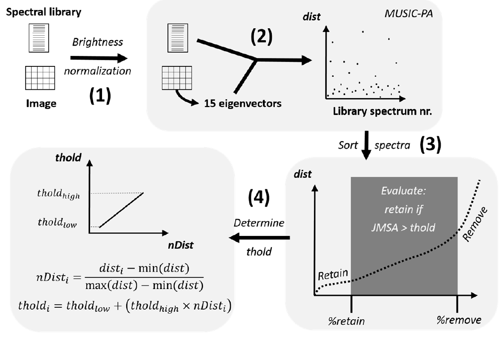
In AMUSES, [Degerickx2017] opted for a spectral separability metric instead of IES to have more control over the entire procedure. A schematic overview of AMUSES is provided in the image below.
The method starts by applying brightness normalization to both the original spectral library and the image, to decrease the effect of brightness during the endmember selection process (step 1 in the figure below). This is accomplished by dividing the reflectance in each band by the average reflectance of the entire signal [Wu2004].
Then MUSIC is used to calculate the distance from each library spectrum to the image (step 2 in the figure below). [Degerickx2017] used a fixed minimum number of eigenvectors (15).The more eigenvectors are retained, the more spectra will be ranked as highly similar to the image and the harder it becomes to identify the true image endmembers.
After ranking all library spectra according to their distance to the image, a fraction of spectra ranked highest are retained and the lowest few are discarded (step 3 in the figure below).
All remaining spectra are assessed one by one using a spectral separability measure: only if a signature is sufficiently dissimilar from the already selected spectra, it will be included in the final selection.
[Degerickx2017] used a metric that combines the Jeffries Matusita distance and Spectral Angle (JMSA) by [Padma2014].
The JMSA threshold is systematically increased. This threshold is used to evaluate the similarity of a candidate spectrum with the already selected spectra (thold parameter in the figure below) in function of the normalized distance of the candidate spectrum to the image as calculated by MUSIC (*nDist in the figure below).
The higher the MUSIC distance, the lower the relevance of a library member to the image being analyzed. By using a high JMSA threshold for these spectra, their chance of ending up in the final selection is decreased. As input to the algorithm, the user needs to define a minimum and maximum threshold between which the thold parameter is allowed to vary.
Using this approach, the pruning algorithm is highly automated as it now decides on the final number of spectra to be retained based on the distance to the image and the mutual similarity of the library spectra.
ACKNOWLEDGMENTS
This user guide is based on the VIPER Tools 2.0 user guide (UC Santa Barbara, VIPER Lab): Roberts, D. A., Halligan, K., Dennison, P., Dudley, K., Somers, B., Crabbe, A., 2018, Viper Tools User Manual, Version 2, 91 pp.
CITATIONS
| [BioucasDias2008] | Bioucas-Dias JM, Nascimento JMP. 2008. Hyperspectral Subspace Identification. IEEE Transactions on Geoscience and Remote Sensing, volume 46, p. 2435-2445. |
| [Clark2005] | (1, 2) Clark M. 2005. An assessment of Hyperspectral and Lidar Remote Sensing for the Monitoring of Tropical Rain Forest Trees. University of California, Santa Barbara, 319 pp. |
| [Degerickx2016] | (1, 2) Degerickx J, Iordache MD, Okujeni A, Hermy M, van der Linden S, Somers B. 2016. Spectral unmixing of urban land cover using a generic library approach. In Proceedings of the SPIE 10008, Remote Sensing Technologies and Applications in Urban Environments, Edinburgh, UK, 26 September 2016. |
| [Degerickx2017] | (1, 2, 3, 4) Degerickx J, Okujeni A, Iordache M-D, Hermy M, van der Linden S, Somers B. 2017. A Novel Spectral Library Pruning Technique for Spectral Unmixing of Urban Land Cover. Remote Sensing, volume 9, 565. |
| [Dennison2003] | Dennison PE, Roberts DA. 2003. The Effects of Vegetation Phenology on Endmember Selection and Species Mapping in Southern California Chaparral. Remote Sensing of Environment, volume 87, p. 295-309. |
| [Dennison2004] | (1, 2) Dennison PE, Halligan KQ and Roberts DA. 2004. A Comparison of Error Metrics and Constraints for Multiple Endmember Spectral Mixture Analysis and Spectral Angle Mapper. Remote Sensing of Environment, volume 93, p. 359-367. |
| [Dudley2015] | Dudley KL, Dennison PE, Roth KL, Roberts DA and Coates AR. 2015. A Multitemporal Spectral Library Approach for Mapping Vegetation Species Across Spatial and Temporal Phenological Gradients. Remote Sensing of Environment, volume 167, p. 121-134. |
| [Fernandez2016] | Fernandez-Manso A, Quintano C and Roberts DA. 2016. Burn severity influence on post-fire vegetation cover resilience from Landsat MESMA fraction images time series in Mediterranean forest ecosystems. Remote Sensing of Environment, volume 184, p. 112-123. |
| [Gardner1997] | Gardner M. 1997. Mapping chaparral with AVIRIS using Advanced Remote Sensing Techniques. University of California, Santa Barbara, 58 pp. |
| [Halligan2002] | (1, 2) Halligan KQ. 2002. Multiple Endmember Spectral Mixture Analysis of Vegetation in the Northeast Corner of Yellowstone National Park. University of California, Santa Barbara, 64 pp. |
| [Iordache2014] | (1, 2, 3) Iordache MD, Bioucas-Dias JM, Plaza A, Somers B. 2014. MUSIC-CSR: Hyperspectral unmixing via multiple signal classification and collaborative sparse regression. IEEE Transactions on Geoscience and Remote Sensing, volume 52, p. 4364-4382. |
| [Padma2014] | Padma S, Sanjeevi S. 2014. Jeffries Matusita based mixed-measure for improved spectral matching in hyperspectral image analysis. International Journal of Applied Earth Observation and Geoinformation, volume 32, p. 138-151. |
| [Quintano2017] | Quintano C, Fernandez-Manso A and Roberts DA. 2017. Burn severity mapping from Landsat MESMA fraction images and Land Surface Temperatures. Remote Sensing of Environment, volume 190, p. 83-95. |
| [Roberts1993] | Roberts DA, Adams JB and Smith MO. 1993. Discriminating Green Vegetation, Non-Photosynthetic Vegetation and Soils in AVIRIS Data. Remote Sensing of Environment, volume 44, p. 255-270. |
| [Roberts1997] | (1, 2) Roberts DA, Gardner ME, Church R Ustin SL and Green RO. Optimum Strategies for Mapping Vegetation using Multiple Endmember Spectral Mixture Models. Proceedings of the SPIE, volume 3118, p. 108-119. |
| [Roberts1998] | Roberts DA, Gardner M, Church R, Ustin S, Scheer G and Green RO. 1998. Mapping Chaparral in the Santa Monica Mountains using Multiple Endmember Spectral Mixture Models, Remote Sensing of Environment, volume 65, p. 267-279. |
| [Roberts2002] | Roberts DA, Numata I, Holmes KW, Batista G, Krug T, Monteiro A, Powell B and Chadwick O. 2002. Large area mapping of land-cover change in Rondônia using multitemporal spectral mixture analysis and decision tree classifiers. Journal of Geophysical Research: Atmospheres, volume 107, p. 40-1 to 40-18. |
| [Roberts2003] | (1, 2) Roberts DA, Dennison PE, Gardner M, Hetzel Y, Ustin SL and Lee C. 2003. Evaluation of the Potential of Hyperion for Fire Danger Assessment by Comparison to the Airborne Visible/Infrared Imaging Spectrometer. IEEE Transactions on Geoscience and Remote Sensing, volume 41, p. 1297-1310. |
| [Roberts2004] | Roberts DA, Ustin SL, Ogunjemiyo S, Greenberg J, Dobrowski SZ, Chen J and Hinckley TM. 2004. Spectral and structural measures of Northwest forest vegetation at leaf to landscape scales, Ecosystems, volume 7, p. 545-562. |
| [Roberts2015] | Roberts DA, Dennison PE, Roth KL, Dudley K and Hulley G. 2015. Relationships Between Dominant Plant Species, Fractional Cover and Land Surface Temperature in a Mediterranean Ecosystem. Remote Sensing of Environment, volume 167, p. 152-167. |
| [Roth2012] | (1, 2) Roth KL, Dennison PE and Roberts DA. 2012. Comparing endmember selection techniques for accurate mapping of plant species and land cover using imaging spectrometer data. Remote Sensing of Environment, volume 127, p. 139-152. |
| [Roth2015] | Roth KL, Roberts DA, Dennison PE, Alonzo M, Peterson SH and Beland M. 2015. Differentiating Plant Species within and across Diverse Ecosystems with Imaging Spectroscopy. Remote Sensing of Environment, volume 167, p. 135-151. |
| [Schaaf2011] | Schaaf AN, Dennison PE, Fryer GK, Roth KL and Roberts DA. 2011. Mapping Plant Functional Types at Multiple Spatial Resolutions using Imaging Spectrometer Data. GIScience Remote Sensing, volume 48, p. 324-344. |
| [Wu2004] | Wu C. 2004. Normalized spectral mixture analysis for monitoring urban composition using ETM+ imagery. Remote Sensing of Environment, volume 93, p. 480-492. |