Exercise: run EAR-MASA-COB in QGIS
Data used
- Spectral Library: roberts2017_urban.sli
Part 1 - EMC
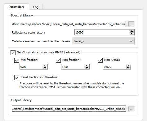
Select the input spectral library.
- Select roberts2017_urban.sli.
- The reflectance scale factor is automatically detected as 10000. This is correct.
- The metadata element we are using for this analysis is Level_7.
Set constraints:
- Minimum fraction to 0.0, maximum to 1.0 and RMSE constraint at 0.025.
- Select the ‘Reset fractions to threshold’ mode.
Output:
- Select a name for the new library, e.g. roberts2017_urban_emc.sli.
Click OK to run EMC.
Result
The following image shows the tabular output of the algorithm (partly).
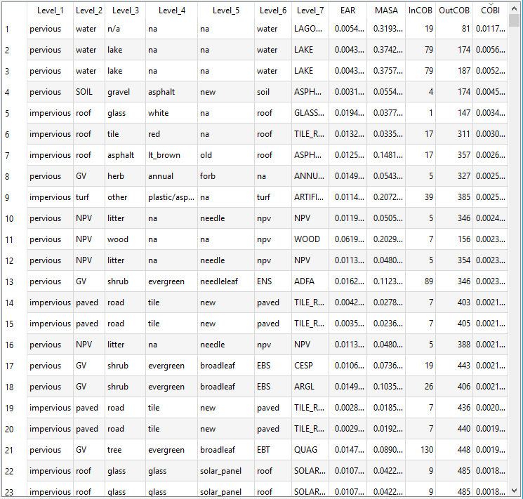
When the metric of choice is Cob, sorting works very well.
The best candidate per Level_7 class is the class with the highest InCob value. In case of a tie, look to other measures (such as EAR) to make your choice.
When the metric of choice is EAR or MASA, this technique is less efficient, as there are many similar RMSE or spectral angles values.
Part 2 - selecting a subset based on the EMC results
Hint
Since these exercises were written, some features were added to the spectral library viewer in order to help the user distinguish between different classes. Think about using different colours for different classes, not displaying certain classes, and only showing selected features on the screen. These features will make this exercise easier to execute than indicated below.
Our objective will be to select the top candidates for each EMC-metric. There are many criteria one could use.
For example, one could select the top three for each metric. Using this approach we would, however, be best served by ensuring the top three all came from different polygons.
Another strategy would be to select the top candidates for EAR, MASA and InCoB. Where more than one InCoB is viable, we would add some until there are too few models left (say 1-3). Using this strategy, we would also remove any duplicates from the same metric, but would also potentially find a tie with InCoB and need another metric to break the tie.
There is no defined way to break the tie, but one option would be the select the one with the lower EAR (this would be the one that fits its class best). Another option would to select the one with the highest EAR (this is the one that is the most distinct from other spectra in the library, and might be a good choice if this were a second InCoB). A third option might be to select one with the lowest OutCoB (Most distinct from other classes).
In this example, we are going to use the strategy of using the top metric for each class, followed by multiple InCoBs. We will split ties by choosing the InCoB with the lowest EAR.
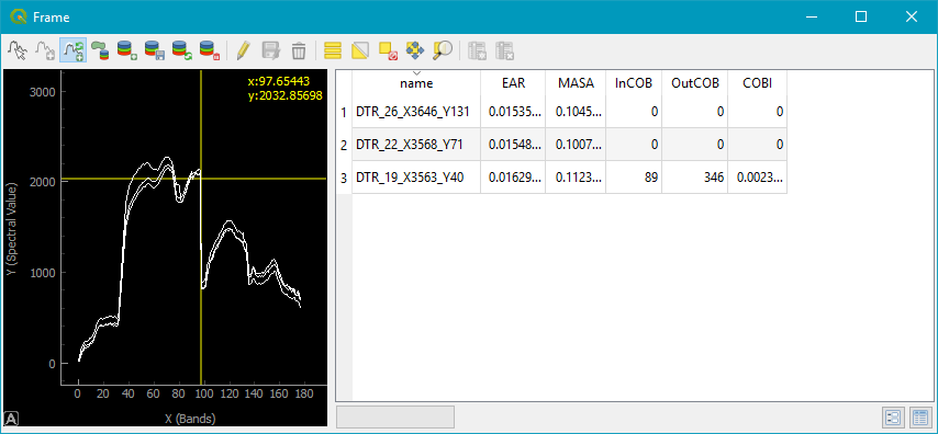
- Order the data according to column 7 and only select ADFA (remove all other spectra - this does not affect the EMC library saved to file).
- Sort by EAR: DTR_26_X3646_Y131 has the lowest EAR value.
- Sort by MASA: DTR_26_X3646_Y131 also has a low MASA value, but is not the best, that is DTR_22_X3568_Y71.
- Sort by InCob: DTR_19_X3568_Y37 and DTR_19_X3572_Y35 both have the highest value (85), but DTR_19_X3568_Y37 has the lowest OutCOB of the two.
- Keep only these tree spectra and save them as a separate library. Afterwards, you can merge all libraries into one.
Repeat this process for all other major classes. As a word of warning, this process can be slow for large libraries.
To work faster, you might opt exporting as CSV and editing in another tool like Excel.
When you are done, merge all sub-libraries again into one by loading them one by one into the Spectral Library viewer and then saving them again to file, e.g. roberts2017_urban_emc_opt.sli*. You should have around 150 spectra when you are done.
Other helpful hints:
Some indices will fail to produce markedly different spectra, even if they come from different polygons. This is particularly true of MASA. It may also not be possible to select more than one candidate from InCoB. If, for example, the third selection models far more of the wrong class than itself, it may be best left out. In addition, because InCoB automatically culls out all spectra from the first selection, even if the second best selection is from the same polygon, it still is likely to be quite different.
Also, keep in mind that you are working with a research tool. Optimal candidates are likely to differ between cover types and data sources. Thus, simply selecting the top three candidates may not be the best option for your study problem.
We do not know all of the answers, but have given you a tool to help you answer yours.
For issues, bugs, proposals or remarks, visit the issue tracker.