Exercise: Run CRES in QGIS
Objective: identify the best set of reference endmembers that unmix chamise, oak, manzanita, Ceanothus, soil and senescent grass with physically reasonable fractions.
Data used
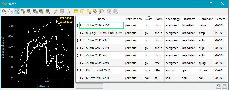
We will start with a spectral library consisting of eight spectra to unmix. These spectra were selected to correspond to nearly pure stands of chamise (adfa: EVF75), big pod Ceanothus (ceme: EVF53), greenbark Ceanothus (cesp: EVF sb poly104), manzanita (argl: EVF52), coast live oak (EVF95) and soil (EVF120). Both senescent grass (EVF133) and senescent chamise (EVF57) are added, to see if we can locate an appropriate NPV that is not senescent grass.
- Library with Image Spectra: viper_tutorial_train_iem.sli
This library consists of laboratory and field spectra originally collected in southern California, Washington state and from libraries developed by the University of Washington. For this example, the library is convolved to the 2001 AVIRIS scene and further subsetted to include only spectra appropriate for Southern California.
- Library for unmixing: 010627_westusa_all.sli
Part 1: Chamise
We will start with chamise (EVF75).
Image Spectrum:
- Select the library viper_tutorial_train_iem.sli.
- Select the spectrum EVF:75_trn_X431_Y64
- The reflectance scale factor is automatically detected as 10000 and can be left that way.
Spectral Library:
- Select the library 010627_westusa_all.sli.
- The reflectance scale factor is automatically detected as 10000 and can be left that way.
- This should result in 1 042 695 models.
- Choose a RMSE threshold for the calculations. This can be left at 0.025.
Calculate SMA Fractions:
- Now the SMA fractions for each of the 1 042 695 models are calculated. This might take a while.
- This step has to be done only once per image spectrum.
You see now a table filed with models: the spectra names and fractions for each class, plus a shade fraction, plus the RMSE. There are 854 198 models in the table and not 1 042 695, because of the RMSE threshold we set earlier.
To limit the table even further, you can filter out absurd results by using the RMSE, Minimum Fraction and Maximum Fraction filters. Mind that with over 800 000 spectra, turning on a filter might also take a few moments. After turning all filters on, xxx models remain.
Calculate Index
Next, we need to estimate the fractions for chamise to allow CRES to search for models that will produce those fractions:
- We start with the following estimation: 50% GV, 0% Soil, 10% NPV and 40% Shade.
The we decide on the weights for the index calculations (see formula):
- Set the weights for the fractions to 1 and the RMSE to 10.
- Click Calculate Index.
- Sort by GV index.
Result for Chamise (adfa)
The best GV index (0.146) leads to a selections of CCEOLSTCK (52% GV, -1% Soil, 9% NPV, 40% Shade, RMSE of 0.014)
We can see that the fractions are nearly identical to our estimates, although the RMSE is a bit high. Given that CCEOLSTCK is an evergreen chaparral leaf spectrum from leaf stacks and cadfa12671 is chamise stems, this is a very good first model.
If we sort on RMSE, we see our best fit is for zsale42I6, generating an RMSE of 0.009, but a physically unreasonable GV fraction of 1.10 (meaning the image endmember is brighter than the spectrum in the library.
Experiment with changing the RMSE multiplier to 5. We can see if we gave RMSE a smaller constraint, we get QUDO1STCK (GV 49%, NPV 10%, Shade 40% and RMSE of 0.016).
Part 2: big pod Ceanothus (ceme)
As a second example, we will see whether this spectrum might also work for ceme.
- Image Spectrum: change the spectrum to EVF:53
- Calculate SMA Fractions: redo the calculations
Looking at EVF53 several things stand out. First, it is much brighter than the other spectra, suggesting a lower shade fraction. Second, it has very low SWIR reflectance, suggesting a low NPV fraction and no soil.
- Calculate Index: fraction estimates: 65% GV, 0% Soil, 5% NPV and 30% Shade
Results for big pod Ceanothus (ceme)
Looking at our first estimate, we find a set of models that produces fractions that match our estimate. In addition, the RMSE is pretty high at 0.021.
We try new fraction estimates: 80% GV, 0% Soil, 0% NPV and 20% Shade
Using this model, we identify CCEOLSTCK as a viable model (78% GV, 1% soil, -3% NPV and 23% shade). However, we find that the RMSE is still poor at 0.024.
This may be our best model, given the library, but we will try one more test. We try new fraction estimates: 65% GV, 0% Soil, 0% NPV and 35% Shade
Our best selection is this case is SASP12STCK (64% GV, 0% soil, 2% NPV and 34% shade). The RMSE is still high at 0.02. This is probably the best we can do, given limitations in the reference library.
Part 3: coast live oak
We will conclude our GV search with coast live oak.
- Image Spectrum: change the spectrum to EVF:95
- Calculate SMA Fractions: redo the calculations
Looking at the spectrum, we can see that it is similar to the chamise spectrum in the NIR, but has lower visible and SWIR reflectance, suggesting lower NPV and slightly higher shade content.
- Calculate Index: fraction estimates: 50% GV, 0% Soil, 0% NPV and 50% Shade
Results for coast live oak
As our first choice, we find selected a Quercus douglasii spectrum. However, we also have several problems, including a high RMS (0.025) and 9% soil fraction.
Sifting down the list we actually see that CCEOLSTK gives better results, with 51% GV, 6% soil and 43% shade. The RMSE for model is better at 0.024 but still fairly high.
From these three experiments, we would conclude that CCEOLSTCK is our best overall model, but still not ideal for this scene because of a high RMSE.
Part 4: senescent grass
- Image Spectrum: change the spectrum to EVF:133
- Calculate SMA Fractions: redo the calculations
Looking at the spectrum, we would suggest a modest shade fraction (20%), minor soil (5%) and no GV.
- Calculate Index: fraction estimates: 0% GV, 5% Soil, 75% NPV and 20% Shade
Results for senescent grass
As our first selection we get u9litt01-av. This is a spectrum of senescent grass measured in the field using an ASD. This model has a very good fit (0.012 RMSE), but requires 17% soil and 20% shade.
While this may be an excellent model, we will try one more by changing the RMSE weight to 5 instead of 10. This has little impact, forcing us to conclude that the soil fraction was probably higher than the initial estimate of 5%.
Part 5: senescent chamise
Next, we will see if we can determine a more appropriate NPV for chamise.
- Image Spectrum: change the spectrum to EVF:57
- Calculate SMA Fractions: redo the calculations
We Looking at this spectrum we can see it is obviously highly mixed, including GV, shade, NPV and probably rock or soil.
Calculate Index: fraction estimates: 25% GV, 15% Soil, 30% NPV and 30% Shade. Keep the RMSE weight at 5.
Results for senescent chamise
As our first pass, we select a fairly reasonable model, consisting of stems from Artemisia calfornica, a soil from the Santa Monica Mountains and leaves from Eriogonum cinarium (an evergreen shrub).
We also see that u9litt01 produces a reasonable model for this spectrum (33% NPV, 22% GV, 15% soil and 30% shade). Given this result, we stick with u9litt01.
Part 6: Soil
We will conclude with a search for a soil spectrum.
- Image Spectrum: change the spectrum to EVF:120
- Calculate SMA Fractions: redo the calculations
Given that this soil is fairly bright, we will start with a low shade fraction of 5%. There is also very little evidence of any senescent material, so we will set the NPV to 0%.
Calculate Index: fraction estimates: 0% GV, 95% Soil, 0% NPV and 5% Shade. Keep the RMSE weight at 5.
Results for Soil
Our first model turns out to be pretty good. We select DCSMM68.DAT (4% shade, 3% NPV and 92% soil). The only negative is a higher RMSE of 0.019.
We can try a second model setting the RMSE weight to 10.
In this case we select J9009181. However, this model also requires a slight negative GV fraction, 105% soil and no shade. DCSMM68.DAT is the better model.
Conclusion
To summarize, we have one GV, NPV and Soil that appear to be reasonable for all of the image endmembers: - CCEOLSTCK (GV) - u9litt01-av (NPV) - DCSMM68.DAT (Soil)
For issues, bugs, proposals or remarks, visit the issue tracker.